These are the results of my foray into Bayesian data analysis applied to a childrens game. This post ties the previous posts concerning simple games, probability theory and functional programming together. After recapping the rules of the particular game I will present the winningest strategy, which will surprise nobody. But I will finish with a plot twist.

Orchard: The Rules of the Game

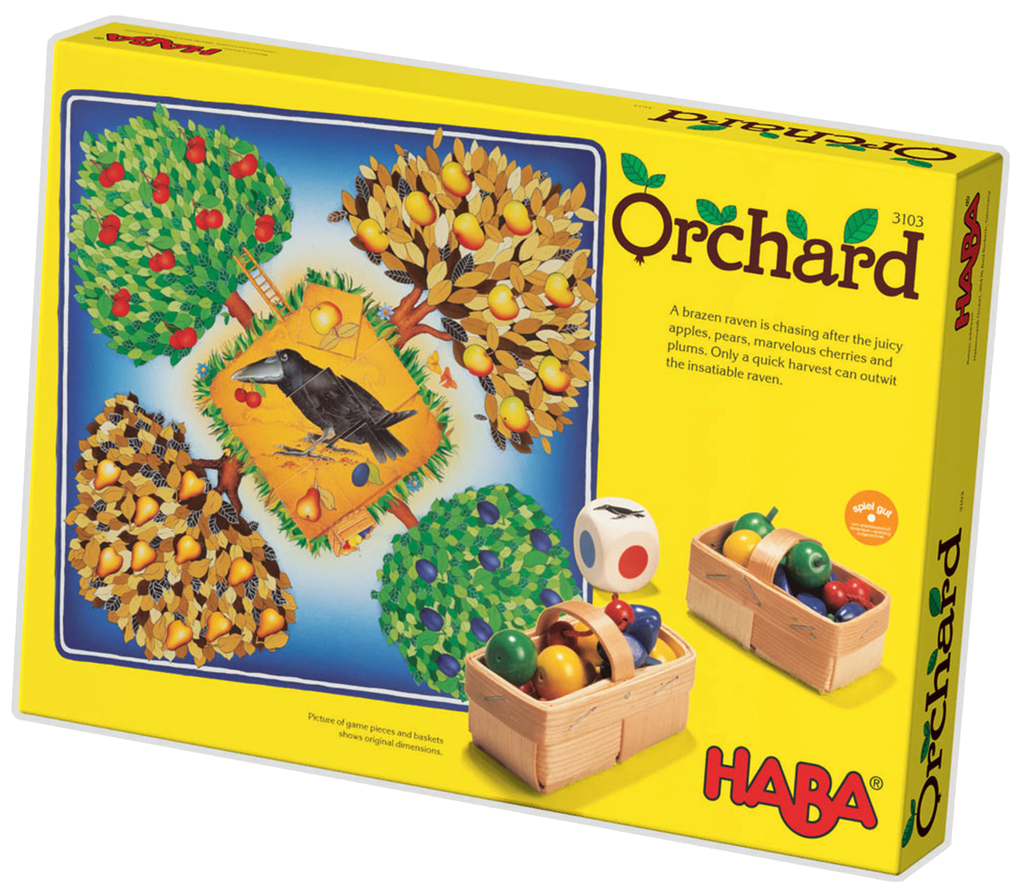
The game I am playing over and over again with my kids is a cooperative game named Orchard by HABA. The players try to pick fruit from a number of trees before a raven gets to the fruit. The main pieces of the game are:

• 10 pieces each of differently colored fruit: blue plums, green apples, yellow pears, red cherries. The fruits are placed on trees on the board.
• 9 raven cards
• and a six sided dice.

Four sides of the dice correspond to the colored fruit. One side depicts a raven, the last side depicts a fruit basket. The rules are simple: The players take turns in throwing the dice. Depending on the result the players take the following actions:

Dice Result	Player Action
Fruit Color	Pick fruit from the respective tree. If the tree is empty, do nothing.
Fruit Basket	Pick two pieces of fuit from any (one or two) trees the player chooses.
Raven	Add a raven card to the middle of the board

The game starts with 40 pieces of fruit and 0 raven cards in the middle. The players lose collectively if the 9^th raven card is placed in the middle. If the players pick all fruit before the raven is complete, they win. The only time the players have agency is when they roll a fruit basket, because they can choose any two fruit from any trees to pick.

It is an exercise in patience watching my kid perpetually ignore the obvious optimal strategy in favor of having fun. That is not how it works! Games should not be fun, they should be rigorously analysed and simulated using overly complex functional programming techniques! Oh… anyways, since the work is done let’s see what I did.

The Question

The strategical element of the game is which fruit the player picks when a fruit basket is rolled. So the obvious question becomes: what is the best strategy? For now, let’s say the best strategy is the one that wins the most. So the question becomes: what is the strategy that produces the highest chance of winning?

Simulating Strategies

I can see four basic strategies from which other strategies could be mixed:

Strategy	Player Action
Pick Greedy	Player picks from the tree(s) with the least (but nonzero) amount of fruit.
Pick Favorite	Player first picks her favorite fruit until it is empty. Then her second favorite fruit and so on.
Pick Random	Player picks from a (truly) random tree.
Pick Fullest	Player picks consecutively from the fullest tree(s).

I wrote a simulation to test the strategies. I made a simplifying assumption to get to the most basic results: All players play the same strategy consistently for the whole duration of the game. The last thing a kid does is play consistent, but I am interested in seeing how the strategies compare concerning their chance of winning.

Results

For a simulated number of \(N=10^7\) games, the results are as follows. Since the result is binary win/loss, I just need to give the number of wins:

Strategy	Number of Wins \(N_W\)	Win Ratio
Pick Greedy	\(5324756\)	\(53.2\%\)
Pick Favorite	\(5685967\)	\(56.9\%\)
Pick Random	\(6320775\)	\(63.2\%\)
Pick Fullest	\(6842964\)	\(68.4\%\)

The data suggests that the Pick Fullest strategy is superior to all other strategies. This is what I assumed but I want to know how confident I can be in these results given the data.

Bayesian Analysis

I am interested in quantifying my knowledge about the chance of winning for each strategy. In part one of this series we introduced the fundamental formulas and the notation. We are interested in the posterior probability \(P(p\vert N_W,N,S,I)\) for the chance of winning \(p\) for each strategy \(S\) given the data \(N_W\), \(N\) and our background knowledge \(I\). This probability is the product of the prior, the likelihood, and a normalization constant. Let’s think about the prior first.

The Prior Distribution

The prior reflects my state of knowledge about the chances of winning. My prior knowledge is anecdotal and unsystematic. In light of \(N=10^7\) experiments the prior is going to have a neglegible influence on the posterior distribution. Thus I just use a uniform prior \(p=const.\) on the interval \((0,1)\) to simplify calculations. If we were operating with less data, then it could pay off to think more carefully about the prior. Questions like: do I really think the prior is independent of strategies? Do I have reasons to believe one strategy is better than the other? Do I honestly think the chances of winning can be close to \(0\) or \(1\) given that this is a childrens game? And so on. We could then have a look at conjugate priors. However, given the amount of data, we’ll just leave it at uniform priors.

Approximating the Likelihood

Because the number of trials is very large, we can approximate the Binomial Distribution with a Gaussian Distribution. This makes it easier to calculate the credible intervals for the chances of winning with a given strategy. In order to prevent cluttering of this post, I placed the calculations in a separate article.

Credible Intervals

To quantify my level of certainty about the data I have calculated the \(5\sigma\) credible interval (CI) for \(p\) with a given strategy. We know that the value of \(p\) is within this interval with a probability of \(99.9999\%\).

Strategy	\(5\sigma\) credible interval for \(p\)
Pick Greedy	[53.17%, 53.33%]
Pick Favorite	[56.78%, 56.94%]
Pick Random	[63.13%, 63.28%]
Pick Fullest	[68.35%, 68.50%]

The Best Strategy … and a Twist

Without even getting into more sophisticated calculations we can be practically certain that the winningest strategy is indeed the Pick Fullest strategy. No surprise there, because that strategy allows the players to even out the distribution of fruit on the trees. Thus, less fruit coloured dice rolls go to waste than in the other scenarios. It is also interesting that the random strategy is so much better than the other two variants. It is also not much worse than the best strategy. However, the difference in outcome is highly significant.

So much for the obvious. I promised to leave you with a twist. I have not only simulated the number of wins and losses but also the number of turns for each strategy. A turn is one roll of the dice. In the future I will look into the Bayesian Analysis of these results, but for now I leave you with the following pieces of information: The average number of turns for the greedy strategy is \(36.4\) and it is the lowest average for all simulated strategies. The average number for the Pick Fullest strategy is highest with \(37.8\) turns. So it turns out that the game pretty much always takes the same time, regardless of strategy. I cannot escape the game by winning or losing fast. It is probably best to see it as an exercise in patience and enjoy the time. After all, it’s time spent with my kids.